Scraping, Clustering, Cleaning and Building a Practice Mode
Author
Nick Tacik
Published
September 24, 2026
Introduction
I like to think of myself as a bit of a Jeopardy aficionado. It’s a ritual for my wife and me to watch an episode as we sit down for lunch or dinner. However, there are definitely some categories that I’m a bit hopeless at — Opera, musicals, Civil War history, biblical names, architecture, and so on. I’d like to get better at these categories, but I’m not even sure where to start.
A hypothesis starts to form as you watch more and more Jeopardy.
There are not really that many total types of categories. The different category types get repeated frequently from game to game.
Within each category there are certain entities that get asked about far more frequently than others.
Those entities often have certain “fingerprints” - specific words used in the clue that signify what the answer is going to be. If I hear “Toreador” in an opera category, I’m betting the answer is “Carmen”, even knowing nothing more about operas.
If I can determine those categories, entities and fingerprints, I’ll have a good basis to study and hopefully get good enough to get on the show one day myself.
In this post, I’ll document my process for building a Jeopardy study tool: scraping the data from J-Archive, clustering the data into types of categories, reconstructing the most common entities in those categories (and the cleaning that goes into it), finding the clue fingerprints for those entities, and finally building the study tool itself.
Scraping the Data
J-Archive does not have an API, so the data comes from a polite, cached crawl.
A fetch stage that does one request per second with every page cached to disk.
A parse stage that reads each game’s board out of the HTML.
A resumable crawl that walks through every season and game.
This is assembled into a single clues.parquet file with one row per clue.
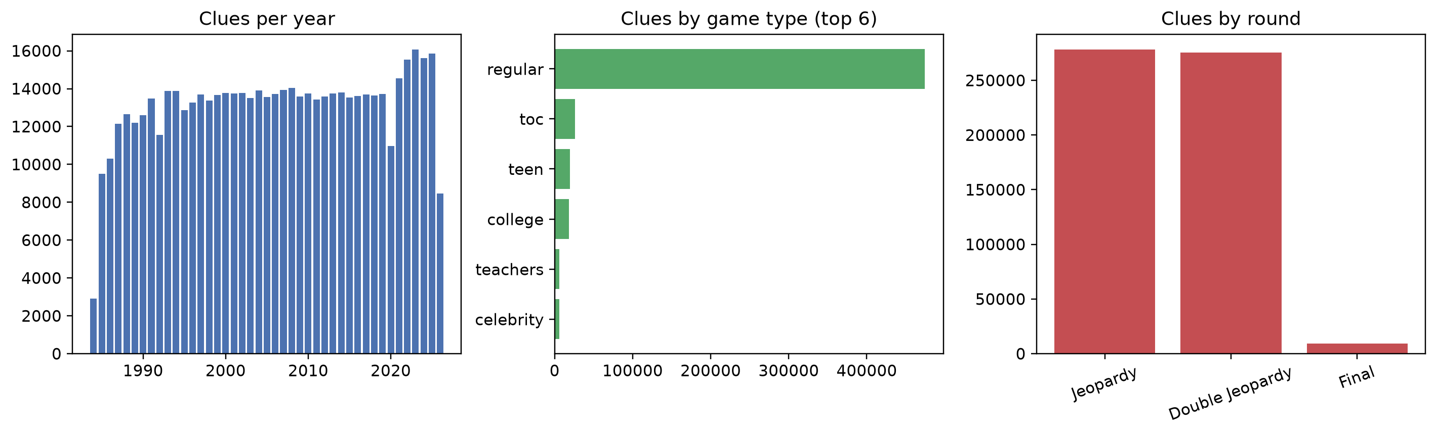
Ultimately, we find 563,266 clues across 9,485 games spanning from 1984 to 2026.
fig, axes = plt.subplots(1, 3, figsize=(13, 4))per_year = clues["air_date"].dt.year.value_counts().sort_index()axes[0].bar(per_year.index, per_year.values, color="#4C72B0")axes[0].set_title("Clues per year")gt = clues["game_type"].value_counts().head(6)[::-1]axes[1].barh(gt.index, gt.values, color="#55A868")axes[1].set_title("Clues by game type (top 6)")rounds = clues["round"].value_counts()axes[2].bar(rounds.index, rounds.values, color="#C44E52")axes[2].set_title("Clues by round")axes[2].tick_params(axis="x", rotation=20)plt.tight_layout()plt.show()
Figure 1: The dataset: clues per year, game types, and rounds.
Clustering in “Types of Categories”
To start clustering, we need to convert each category into a short “document”. The choice here is to take the category title, followed by its clue → answer pairs in a shuffled order (so no clue’s position carries special weight).
Each document is embedded into a 384-dimensional vector with a local sentence-transformer (bge-small-en-v1.5). This step is run offline and commits its output once.
NoteRunning a sentence-transformer locally
A sentence-transformer turns a chunk of text into a fixed-length vector where semantically similar texts land near each other. bge-small-en-v1.5 is a small, fast one (384 dimensions) that runs comfortably on a CPU. With the sentence-transformers library it’s essentially two lines:
from sentence_transformers import SentenceTransformermodel = SentenceTransformer("BAAI/bge-small-en-v1.5")vectors = model.encode(documents, batch_size=64, show_progress_bar=True)
The model downloads once (~130 MB) and then embeds entirely offline — no API, no per-call cost. Encoding the ~123k category documents takes a few CPU-only minutes, which is exactly why it runs once and commits its output rather than re-running on every build.
Running K-means (k = 50) over those vectors groups the ~123k category instances into recognizable types. Projected to 2D with UMAP, the map looks like Figure 2. Hover any point to see its type, an example category, and that type’s most common entity. I chose the hyperparameter k=50, with a bit of experimentation. When k was too low, US presidents got merged together with Geography, but when it was too high, it was a bit too hard to interpret the meaningful differences between the categories.
NoteUMAP
UMAP (Uniform Manifold Approximation and Projection) is a nonlinear dimensionality-reduction technique — it squashes the 384-dimensional embeddings down to 2D while trying to keep nearby points nearby, purely so we can see the structure. The clustering itself (K-means) runs on the full 384-dimensional vectors; UMAP is only for drawing this picture.
Figure 2: 123k category instances, grouped into 50 types (hover to explore; ~4.5k-point sample).
This methodology assumes a category can be neatly clustered, which isn’t always true. Picture a category whose only through-line is that every answer’s last name is “Johnson” — those Johnsons might come from politics, sports, and the arts all at once. Because the unit of clustering is the whole category (not the individual clue), such a category isn’t torn apart; it’s embedded as one document and assigned wherever its overall text points. And categories that don’t sit near any clean type aren’t dropped — the worst ~5% by distance to their cluster’s centre are swept into a synthetic 51st type, Misc: Hard to Classify.
The 50 types are also far from equal in size — Table 1 lists all of them, sorted by how many category instances each contains. The largest few (two flavours of wordplay, plus music, books, and movies) are also the broadest and most conceptually loose.
To name each of the 50 types, each cluster gets an automatic three-part summary — its most frequent real category names, the instances closest to its centre, and its most distinctive words (via TF-IDF over the pooled category text — see below). That summary is handed to an LLM (gpt-4o-mini), which returns a short 2–4 word name for each; the names are committed to a CSV the pipeline only reads, so nothing calls the model at build time.
NoteHow the “distinctive words” are scored
To find each type’s signature vocabulary, I pool all of a type’s categories into one big document — 50 documents, one per type — and run an ordinary TF-IDF (Term-Frequency–Inverse-Document-Frequency) over them. A word scores high for a type when it’s frequent inside that type (the TF part) but appears in few of the 50 pooled documents (the IDF part). So inaugural, which lives almost entirely in one type, floats to the top, while a word spread across many types gets downweighted — with scikit-learn’s smoothed IDF, log((1 + n) / (1 + df)) + 1, ubiquitous words are pushed down but never fully cancelled to zero.
(This is the plain-vanilla version. BERTopic popularized a “class-based” c-TF-IDF with a different reweighting designed exactly for this pool-per-class setup; I stuck with stock scikit-learn TF-IDF, which is simpler and good enough to read a name off of.) The same idea, pointed at a single answer instead of a whole type, is how the clue fingerprints below are built.
Table 1: The 50 category types, ranked by number of category instances, with example entities.
Type
Categories
Example entities
0
Wordplay & Vocabulary
5064
Latin, Greek
1
Pop Music & Songs
4230
Beatles, Grammy
2
Books & Authors
4113
Pulitzer Prize, Charles Dickens
3
Rhymes, Anagrams & Common Bonds
4077
Shakespeare, God
4
Movies
3773
Oscar, Disney
5
Notable People & Awards
3760
Supreme Court, White House
6
Word Origins & Foreign Words
3669
Latin, Greek
7
Food & Drink
3426
France, Italy
8
U.S. Geography
3344
California, Texas
9
Animals & Zoology
3124
Australia, South America
10
Literature & Fictional Characters
3111
Charles Dickens, Moby Dick
11
World Geography & Waters
3100
Canada, South America
12
American History
2987
Union, Virginia
13
Television
2979
Emmy, Michael J. Fox
14
Potpourri / Grab-Bag
2911
Christmas, Guinness
15
World History & Leaders
2858
France, China
16
Museums, Landmarks & Travel
2828
London, Washington
17
Puzzle & Grab-Bag Categories
2825
Earth, God
18
Royalty & European History
2794
England, France
19
Oscars & Movie Quotes
2713
Oscar, James Bond
20
Names & Nicknames
2702
Oscar, Abraham Lincoln
21
Countries & Languages
2654
India, France
22
U.S. Presidents
2631
Senate, Richard Nixon
23
Sports
2425
World Series, New York Yankees
24
Medicine & The Body
2395
Latin, Greek
25
Law, Economics & Abbreviations
2222
Latin, Congress
26
Fashion & Furnishings
2186
Christian Dior, China
27
Religion & The Bible
2172
Jesus, God
28
World Capitals & Cities
2094
Canada, Paris
29
Explorers & Ships
2094
Canada, Christopher Columbus
30
Business & Brands
2067
Procter & Gamble, Johnson & Johnson
31
Chemistry & Earth Science
2050
Earth, Sun
32
Opera & Classical Music
2046
Mozart, Beethoven
33
Children's Literature
1936
Alice, Disney
34
TV Sitcoms & Families
1930
Emmy, Fox Broadcasting Company
35
Famous Women & First Ladies
1880
Susan B. Anthony, White House
36
Quotes & Proverbs
1825
God, Plato
37
Inventors & Scientists
1755
Nobel Prize, Thomas Edison
38
Mythology & The Ancient World
1704
Zeus, Rome
39
Theatre & Broadway
1605
Broadway, Tony Award
40
Poetry
1602
Robert Frost, John Keats
41
Plants & Botany
1598
Japanese, Christmas
42
Art & Artists
1592
Pablo Picasso, Leonardo da Vinci
43
Games & Play
1489
Olympic Games, Monopoly
44
Transportation & Cars
1349
Ford, Chevrolet
45
Astronomy & Space
1194
Earth, Mars
46
Holidays & The Calendar
1154
Christmas, Easter
47
Math & Measurement
1082
Earth, Celsius
48
Colleges & Universities
952
Harvard, William & Mary
49
Shakespeare
883
Hamlet, William Shakespeare
Where is the Study Material?
Wordplay seems to be a big, unusual slice. The two pure letter/anagram types - Wordplay & Vocabulary and Rhymes, Anagrams & Common Bonds - are 7.4% of all categories between them, and folding in Word Origins & Foreign Words brings the wordplay-and-language family to 10.4%, about one category in ten. It’s unusual because it rewards a skill you can drill through repetition more than the facts you memorize. It also splits into two tracks — pure letter games versus the genuinely studyable etymology and idioms.
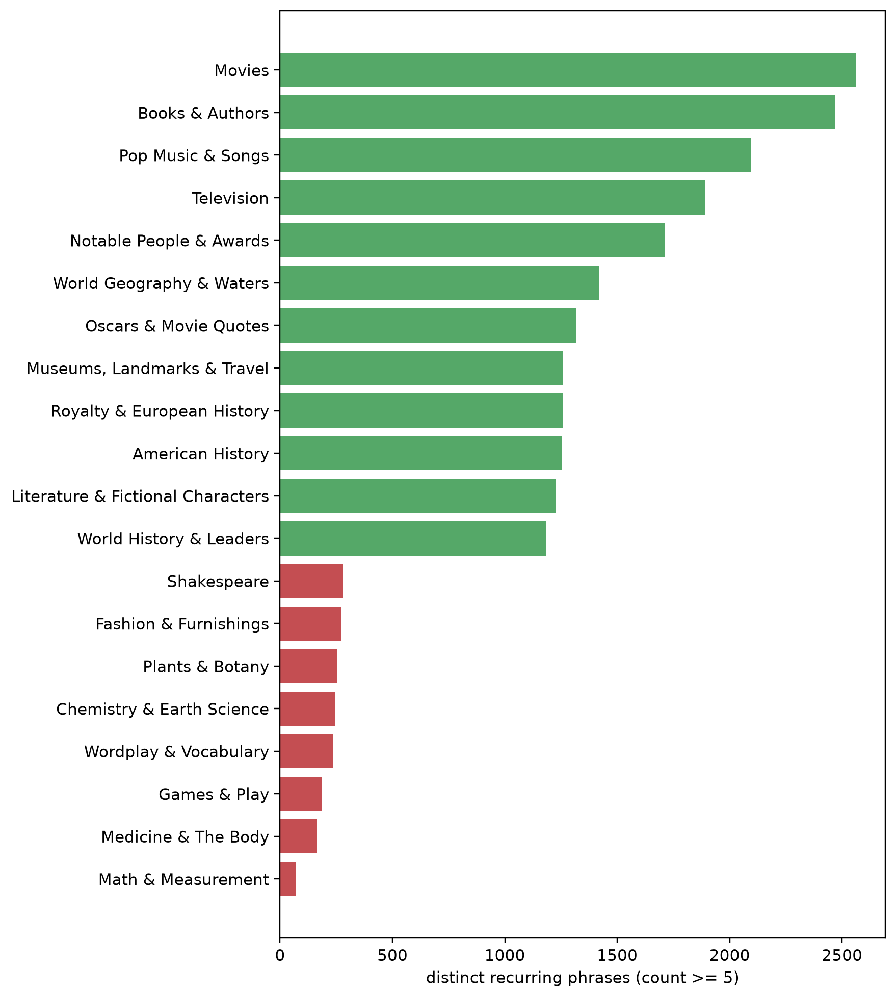
Types differ quite a bit in how much recurring material they even offer — and if a type has little of it, my whole hypothesis about studyability falls apart. As a rough gauge, I count how many distinct phrases recur 5 or more times in a type, drawn from both clues and answers. It really is rough: the phrases aren’t cleaned yet (so stray first names, presenters, and near-duplicates are all still counted), and breadth isn’t payoff — a phrase repeating a lot doesn’t prove that studying it is worth your time.
Figure 3: Breadth of recurring material: distinct phrases (from clues and answers) recurring 5+ times, per type.
And for the material-rich types, here are the phrases that recur most, counted across clues and answers. These recurring names give me a concrete starting list to study — a ranked “if this type comes up, know these.” (They’re truncated mention counts, not a coverage calculation, so I won’t claim what fraction of a type’s clues they account for — just that they come up a lot.)
Table 2
U.S. Presidents
count
0
Senate
363
1
Richard Nixon
315
2
Ronald Reagan
266
3
Abraham Lincoln
249
4
George Washington
241
5
Theodore Roosevelt
219
6
Harry Truman
211
7
Congress
211
8
White House
192
9
Gerald Ford
189
World Geography & Waters
count
0
Canada
473
1
South America
345
2
Africa
293
3
Australia
260
4
Mediterranean Sea
228
5
Italy
197
6
Pacific
196
7
Europe
196
8
France
196
9
Atlantic
195
Books & Authors
count
0
Pulitzer Prize
259
1
Charles Dickens
249
2
Ernest Hemingway
201
3
Mark Twain
180
4
Sinclair Lewis
167
5
John Steinbeck
151
6
Edgar Allan Poe
144
7
F. Scott Fitzgerald
126
8
Nathaniel Hawthorne
123
9
William Faulkner
123
Cleaning the Data
To actually make sense of the data, we need to clean it up. Hand-written regex rules get a lot of the way there, but there are a lot more judgment calls to make that require interpreting the context. Is “John” a studyable entity or a stray first name? John Adams is studyable, John isn’t. Is “May” the month or “Theresa May”? “Sarah of the Clue Crew” comes up a lot, but that’s just a clue presenter, not a studyable entity.
With this in mind, the lists were handed off to an LLM for a second look. For each type, it judged every candidate entity - keep, drop, or merge into a canonical form - with the type’s context in view. It dropped the noise (bare first names, nationalities like “British”, months, Clue Crew presenters, etc.) and stitched fragments back together - “Grey” + “Anatomy” -> “Grey’s Anatomy”. These verdicts live in a committed CSV that the pipeline only reads, so the render stays deterministic.
A second cleaning pass asks a sharper question - not just “is this a real entity” but “does it belong to this topic?”. This was able to pull valid but off-topic answers out of the wrong lists. For example, “New York City” is a fine entity, but it belongs in, say, Geography not in Books & Authors, so it no longer clutters the authors list.
The Study Tool
The study tool is live at research/. Pick a category type, see its most common (cleaned) entities, and jump straight to Wikipedia for each.
It’s filterable by a cumulative window - all-time or restricted to clues aired since 1990, 2000, 2010, 2020. This lets you see how a type’s recurring entities shift as you narrow to more recent years.
The Sample Clue button draws a real clue from that category. Optionally, if an entity is highlighted, it will draw a clue related to that entity.
Clue Fingerprints: For each entity, we look for the handful of terms that Jeopardy keeps reusing to ask about that entity, showing an N-of-M count of how many of that answer’s clues the term shows up in, plus real example clues. Tap a cue, and, where it could be pre-computed, a one-sentence note explains why that word points at the answer. The cues were found using the same TF-IDF trick from naming, but pointed at a single answer instead of a whole type. Filters do the rest of the work - drop the answer’s own name, throw out type-generic terms that show up across most of the type’s answers, and require a cue to appear in at least two of the answer’s clues.
For actual drilling, there’s a Practice mode: pick your topics and it deals you a run of distinct real clues, one at a time with the answer hidden, then a quick tally at the end. (Text-only, so it skips clues that lean on an image or audio you can’t see.)